Piezoelectric Constant Testing for Materials

Piezoelectricity is a fundamental electromechanical phenomenon exhibited exclusively by non-centrosymmetric crystalline solid materials. Out of the 32 classical crystallographic point groups, exactly 21 lack a center of inversion symmetry, and 20 of these exhibit direct piezoelectricity (with the cubic point group 432 being an exception due to higher geometric symmetry). In these crystal classes, mechanical stress induces asymmetric internal displacement of positive and negative ion sublattices, generating macroscopic electric polarization.

Accurately evaluating the complete electromechanical tensor of piezoelectric materials is essential for transducer design, sensor calibration, and acoustic imaging. However, a common source of confusion in industrial metrology is conflating different piezoelectric tensor constants—specifically the piezoelectric charge coefficient (dij), piezoelectric voltage coefficient (gij), electromechanical coupling factor (kij), and mechanical quality factor (Qm). Each parameter represents a distinct thermodynamic state variable with specific measurement boundary conditions. Establishing accurate metrology requires a complete tensor reference framework based on international standards.

Thermodynamic Constitutive Equations and Tensor Coordinate Definitions

Piezoelectric behavior couples mechanical stress (Tkl), mechanical strain (Sij), electric field (Ek), and dielectric displacement (Di). According to IEEE Std 176, the coupled system is described by four interrelated linear constitutive equations depending on the chosen independent thermodynamic variables:

d-Formulation:
Sij = sijklE · Tkl + dkij · Ek
Di = dikl · Tkl + εikT · Ek

g-Formulation:
Sij = sijklD · Tkl + gkij · Dk
Ei = −gikl · Tkl + βikT · Dk

e-Formulation:
Tij = cijklE · Skl − ekij · Ek
Di = eikl · Skl + εikS · Ek

where sijkl is elastic compliance, cijkl is elastic stiffness, εik is dielectric permittivity, βik is dielectric impermeability, and the superscripts E, D, T, and S designate constant electric field (short-circuit), constant electric displacement (open-circuit), constant stress (mechanically free), and constant strain (mechanically clamped), respectively.

Using compressed Voigt matrix notation (contracting tensor indices 11→1, 22→2, 33→3, 23→4, 13→5, 12→6), the third-order piezoelectric charge tensor dkij is represented as a 3 × 6 matrix. For poled polycrystalline ceramics and wurtzite crystals possessing transverse isotropy (point group ∞mm or 6mm), the matrix simplifies to five non-zero components, of which only three are independent:

Matrix Form	Component 1	Component 2	Component 3	Component 4	Component 5	Component 6
Row 1 (E1)	0	0	0	0	d15	0
Row 2 (E2)	0	0	0	d15	0	0
Row 3 (E3)	d31	d31	d33	0	0	0

The voltage coefficient gij, which quantifies the electric field generated per unit of mechanical stress under open-circuit conditions, relates to dij through dielectric permittivity:

g33 = d33 / ε33T = d33 / (ε0 · εr33)

g31 = d31 / ε33T = d31 / (ε0 · εr33)

For hydrostatic acoustic sensors subjected to uniform triaxial pressure (T1 = T2 = T3 = −p), the hydrostatic charge coefficient dh and hydrostatic voltage coefficient gh govern performance:

dh = d33 + 2 · d31

gh = dh / (ε0 · εr33)

Hydrostatic sensitivity figure of merit (FOM) is defined as the product dh · gh (expressed in 10⁻¹⁵ m²/N).

Complete Piezoelectric Parameter Metrology Cheat-Sheet

Materials engineers and transducer designers require clear definitions of units, boundary conditions, and test methods for each tensor component.

The reference matrix below outlines definitions, standard specimen geometries, and measurement methods across the primary piezoelectric parameters:

Parameter Symbol	Formal Parameter Name	Standard SI Units	Physical Significance	Standard Specimen Geometry (IEEE 176)	Primary Measurement Metrology
d33	Longitudinal charge coefficient	pC/N or m/V	Charge per force along poling axis; longitudinal displacement	Thick circular disc or cylinder (t > 1 mm, D/t < 5)	Quasi-static Berlincourt method or dynamic force
d31	Transverse charge coefficient	pC/N or m/V	Charge along poling axis per transverse stress	Slender rectangular bar (L » W, T; L/T > 10)	IEEE transverse length-extensional resonance
d15	Shear charge coefficient	pC/N or m/V	Charge perpendicular to poling axis per shear stress	Rectangular plate with shear poling orientation	Thickness-shear impedance resonance
g33	Longitudinal voltage coefficient	× 10⁻³ V·m/N	Electric field per unit stress under open circuit	Thick circular disc or cylinder	Calculated: g33 = d33 / (ε0 · εr33)
kp	Planar electromechanical coupling	Dimensionless (0 to 1)	Energy conversion ratio in radial breathing mode	Thin circular disc (D/t > 10, D ≈ 20–25 mm)	Radial resonance-antiresonance frequencies
kt	Thickness electromechanical coupling	Dimensionless (0 to 1)	Energy conversion ratio in pure thickness mode	Thin plate with laterally clamped boundaries	Thickness extensional resonance spectrum
Qm	Mechanical quality factor	Dimensionless	Ratio of stored acoustic energy to energy dissipated per cycle	Slender bar or radial disc at fundamental resonance	3 dB bandwidth: Qm = fr / (f2 − f1)

Coupling Factor Extraction via IEEE Std 176 Resonance Method

While charge coefficients (dij) can be measured quasi-statically, electromechanical coupling factors (k) and mechanical quality factors (Qm) are extracted dynamically via acoustic resonance under IEEE Std 176 and IEC 60483.

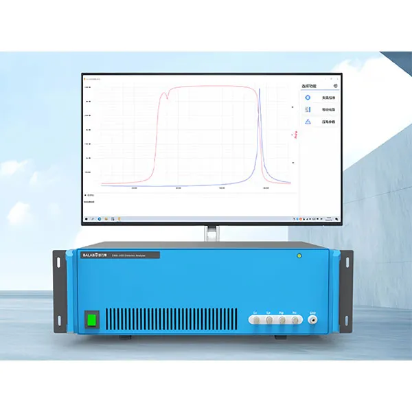
By sweeping frequency across an electromechanical resonance, an impedance analyzer acquires the minimum impedance frequency (resonance, fr) and maximum impedance frequency (antiresonance, fa). For a thin disc operating in fundamental planar radial vibration, the planar coupling factor kp is calculated from the Onoe transcendental equation or its established polynomial approximation:

kp ≈ [(2.51 · (fa − fr) / fr) − (1.07 · (fa − fr) / fr)²]0.5

Similarly, the thickness-extensional coupling factor kt of a thin plate is extracted from:

kt = [(π / 2) · (fr / fa) · tan((π / 2) · (fa − fr) / fa)]0.5

The mechanical quality factor Qm, which dictates acoustic transducer heating and bandwidth, is calculated using the minimum impedance magnitude |Zm| at resonance:

Qm = fa² / [2 · π · fr · |Zm| · C0 · (fa² − fr²)]

where C0 is the clamped (high-frequency) electrostatic capacitance.

The comparative table below summarizes electromechanical coupling and quality factor values across representative material classes:

Piezoelectric Material Class	Typical Composition	Planar Coupling kp	Thickness Coupling kt	Longitudinal d33 (pC/N)	Mechanical Quality Qm	Dielectric Constant εr33
Soft PZT Ceramics	PZT-5A / PZT-5H	0.60–0.68	0.48–0.52	450–650	65–80	1700–3400
Hard PZT Ceramics	PZT-4 / PZT-8	0.52–0.58	0.46–0.50	220–320	500–1200	1000–1400
Lead-Free Piezoceramics	KNN-based / BNT-based	0.38–0.48	0.35–0.42	120–200	100–300	600–1200
Piezoelectric Single Crystals	PMN-PT (Relaxor-PT)	0.85–0.92	0.58–0.62	1500–2500	80–150	4500–7000
Wurtzite Sputtered Thin Films	AlN / Sc0.2Al0.8N	N/A (Clamped)	0.25–0.35	5–15	800–2000	9–14

Comprehensive Parameter Metrology with the MatMeas PCA-1000 System

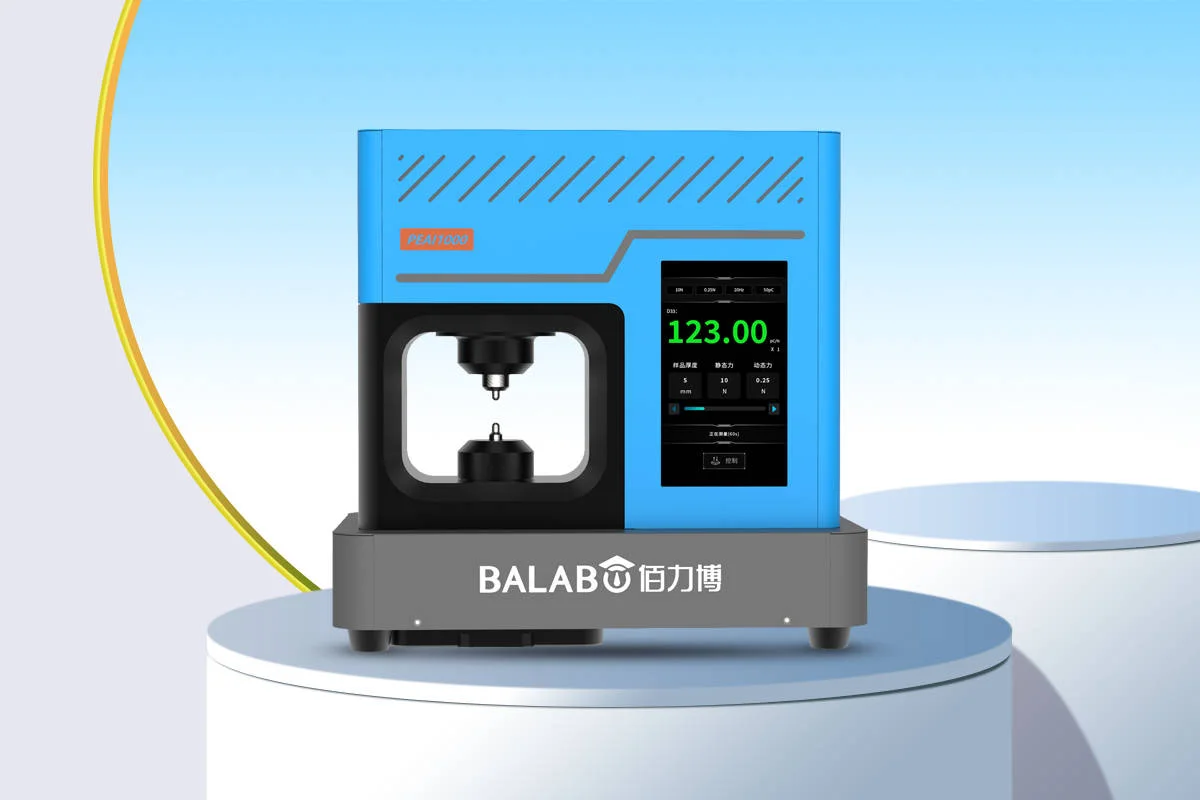
Characterizing the complete electromechanical matrix requires instrumentation that seamlessly bridges quasi-static direct force testing with high-frequency dynamic resonance impedance analysis. The MatMeas PCA-1000 Piezoelectric Parameter Analyzer provides an integrated testing platform engineered specifically for comprehensive piezoelectric metrology.

The PCA-1000 combines a high-precision Berlincourt quasi-static test head (calibrated at 110 Hz with automated pneumatic preload regulation) and an internal multi-frequency impedance engine. This integrated architecture allows users to insert a single ceramic disc and sequentially extract longitudinal d33, radial resonance spectra (fr, fa), planar coupling factor kp, thickness coupling factor kt, dielectric constant εr, dielectric loss tan δ, and mechanical quality factor Qm within seconds. Automated calculation routines apply full IEEE Std 176 polynomial corrections, eliminating manual calculation errors and ensuring full calibration traceability.

Frequently Asked Questions

What is the fundamental physical difference between d33 and g33?

The charge coefficient d33 (expressed in pC/N or m/V) quantifies the electric charge generated per unit of applied force under short-circuit electrical conditions (E = 0), or the strain generated per unit electric field under zero mechanical stress. It is the primary metric for actuators and high-power ultrasound. The voltage coefficient g33 (expressed in V·m/N) quantifies the open-circuit electric field developed across the material per unit of applied mechanical stress (D = 0). Because g33 = d33 / (ε0 · εr), materials with modest d33 but very low dielectric constant (such as PVDF polymer or lead metaniobate) exhibit exceptionally high g33 values, making them superior for passive voltage-sensing hydrophones and impact sensors.

Why does a high d33 material not always make the best ultrasonic transducer?

While a high d33 enhances transmission acoustic output, receiver performance depends on the voltage coefficient g33, and overall transducer efficiency is governed by the electromechanical coupling factor kt or k33. Furthermore, high-power therapeutic or surgical transducers require high mechanical quality factors (Qm > 1000) and low dielectric loss (tan δ < 0.5%) to prevent internal thermal runaway. Soft PZT ceramics possess high d33 (~500 pC/N) but have low Qm (~70), causing them to overheat rapidly under continuous resonance, whereas hard PZT (d33 ~250 pC/N, Qm ~1000) delivers superior continuous acoustic power without depoling.

How is the mechanical quality factor Qm determined from an impedance curve?

The mechanical quality factor Qm represents the ratio of stored elastic mechanical energy to energy dissipated per vibration cycle. In an acoustic impedance spectrum measured around fundamental resonance, Qm is extracted either via the 3 dB bandwidth method: Qm = fr / (f2 − f1), where f1 and f2 are frequencies where conductance falls to half its peak value, or from the minimum impedance magnitude |Zm|: Qm = fa² / [2 · π · fr · |Zm| · C0 · (fa² − fr²)]. A sharper, deeper impedance valley indicates lower mechanical damping and a higher Qm.