Ferroelectric Hysteresis Loop Testing: Circuits, Parameters, and Good Practice
Technical News
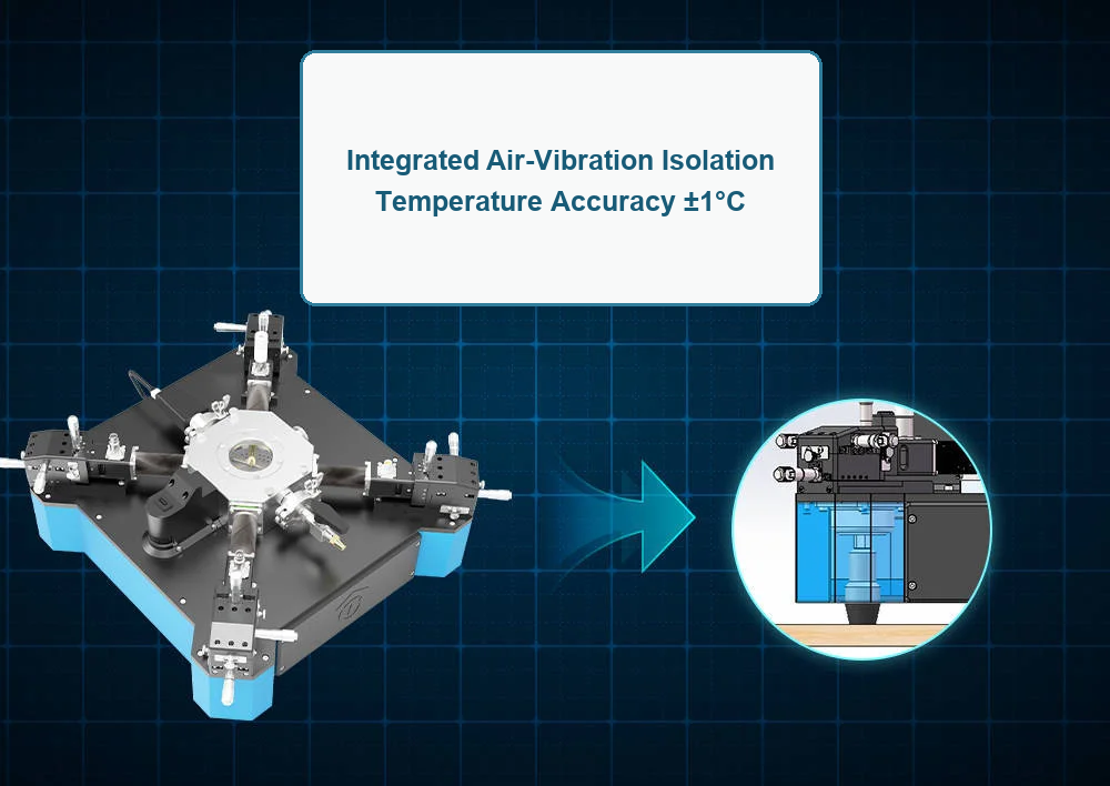
Polarization-electric field (P-E) hysteresis loop measurement is the foundational characterization technique for evaluating ferroelectric materials. Originating from the non-centrosymmetric crystalline structure of ferroelectrics, spontaneous polarization can be reoriented between bistable states by an externally applied electric field. A properly acquired P-E loop provides a complete electromechanical and thermodynamic profile, quantifying switchable remanent polarization (P_r), saturation polarization (P_s), coercive field (E_c), internal imprint bias fields, domain switching velocity, and electrostatic energy storage efficiency.
However, in the field of materials physics, few experimental techniques are as prone to misinterpretation as P-E loop tracing. A hysteretic, closed loop displayed on an oscilloscope or computer screen is not definitive proof of ferroelectricity. Finite dielectric conductivity, non-linear space-charge accumulation, electrode Schottky barrier leakage, and test circuit phase shifts frequently generate closed loops that mimic genuine ferroelectricity in materials that possess zero spontaneous polarization.
To establish rigorous laboratory metrology adhering to IEEE Std 180 and ASTM F668, researchers must understand the circuit theory separating historical passive circuits from modern active architectures, apply rigorous constitutive equations, diagnose artifacts, and enforce strict experimental controls.
Circuit Architectures: Sawyer-Tower vs. Modern Virtual-Ground Transimpedance Systems
To extract the electrical polarization P(t) of a material, an instrument must measure the transferred charge Q(t) traversing the specimen under a cyclic excitation voltage V_in(t), normalizing charge by the active capacitor electrode area A (P = Q / A). Two primary circuit topologies exist to accomplish this task.
1. The Classical Sawyer-Tower Passive Circuit
Invented in 1930, the Sawyer-Tower circuit remains a classic teaching topology due to its simplicity. A known, linear reference sensing capacitor C_sense is placed in series with the ferroelectric specimen under test (DUT, capacitance C_x). A high-voltage AC source V_in(t) is applied across the series combination:
-
The voltage across the sensing capacitor V_sense(t) is monitored:
Q(t) = C_sense * V_sense(t)
P(t) = Q(t) / A = [C_sense * V_sense(t)] / A
While straightforward, the Sawyer-Tower circuit suffers from major metrological limitations:
-
Voltage Division Error: The actual voltage dropped across the ferroelectric specimen V_sample(t) is reduced by the voltage across the sense capacitor:
V_sample(t) = V_in(t) - V_sense(t)
E(t) = [V_in(t) - V_sense(t)] / d
To minimize this distortion, C_sense must be chosen much larger than C_x (typically C_sense >= 100 * C_x to 1000 * C_x), which severely attenuates the output voltage V_sense to millivolts, degrading the signal-to-noise ratio.
-
Phase Shift Distortion: The series combination of a lossy sample resistor-capacitor network with C_sense introduces an intrinsic phase lag, creating artificial loop opening that mimics remanent polarization.
-
Parasitic Cable Capacitance: Stray capacitances of coaxial test cables shunt C_sense, causing direct calibration errors.
2. Modern Active Virtual-Ground Transimpedance Amplifier (TIA) Circuit
Modern research-grade ferroelectric analyzers reject passive capacitive dividers in favor of an active virtual-ground transimpedance amplifier (current-to-voltage converter) topology.
The drive voltage V_in(t) is applied to the top electrode of the specimen, while the bottom electrode connects directly to the inverting input (-) of an ultra-low-bias operational amplifier. The non-inverting input (+) is tied to ground. Because negative feedback forces the inverting terminal to remain at virtual ground (V_inv approx 0 V):
-
The voltage across the specimen is strictly identical to the applied excitation voltage:
V_sample(t) = V_in(t)
E(t) = V_in(t) / d
Zero voltage division occurs, guaranteeing that the programmed electric field waveform is delivered to the material without distortion.
-
The instantaneous current I_sample(t) flowing through the specimen is forced through a precision feedback resistor R_feedback:
V_out(t) = -I_sample(t) * R_feedback
I_sample(t) = -V_out(t) / R_feedback
-
The polarization charge Q(t) is obtained via high-speed, mathematically calibrated numerical integration:
Q(t) = integral_0^t I_sample(t') dt' = - (1 / R_feedback) * integral_0^t V_out(t') dt'
P(t) = Q(t) / A = [1 / (A * R_feedback)] * integral_0^t -V_out(t') dt'
Holding the low-potential electrode at virtual ground completely eliminates the influence of cable capacitance, provides a vast dynamic range across six decades of current, and enables digital leakage compensation algorithms.
Architectural Comparison: Sawyer-Tower vs. Virtual-Ground TIA
The operational capabilities and error profiles of both circuit paradigms are compared in the table below.
| Architectural Feature | Classic Sawyer-Tower Passive Integrator | Modern Virtual-Ground Transimpedance Analyzer (TIA) |
|---|---|---|
| Circuit Type | Passive capacitive voltage divider (DUT in series with C_sense) | Active feedback electrometer (DUT tied to virtual ground op-amp) |
| Voltage Drop Across Specimen | Distorted; V_sample = V_in - V_sense (reduces field by 1% to 15%) | Pristine; V_sample = V_in (zero voltage drop across ground terminal) |
| Phase Lag & Instrumental Error | High; series RC network introduces artificial phase opening | Negligible; phase-compensated operational amplifier up to 100 kHz |
| Low-Charge Sensitivity | Poor; small charges produce sub-millivolt signals on large C_sense | Exceptional; resolves charges down to 0.01 pC using switchable gain |
| Cable Capacitance Immunity | Low; coaxial cable capacitance directly parallels C_sense | Complete; cable shield and core are at virtual ground equipotential |
| Frequency Bandwidth | Narrow; restricted by RC time constant of C_sense and scope probe | Ultra-wide; DC up to 250 kHz with high-speed digital integration |
| Dynamic Leakage Decoupling | Impossible; analog capacitor integrates all currents indiscriminately | Enabled; digital current waveform analysis permits DLCC algorithms |
| High-Voltage Breakdown Safety | Vulnerable; sample puncture discharges full HV directly into scope | Integrated microsecond crowbar clamping isolates sensitive electrometer |
Constitutive Equations and Energy Storage Metrics
The total current density J_total(t) traversing a dielectric under a time-varying electric field E(t) consists of displacement current and conductive leakage current:
J_total(t) = dD/dt + J_leak(E(t)) = epsilon_0 * epsilon_r * (dE/dt) + dP/dt + sigma(E) * E(t)
Where:
- epsilon_0 * epsilon_r * (dE/dt): The linear dielectric displacement current arising from electronic and ionic lattice polarization.
- dP/dt: The non-linear ferroelectric domain switching current, which peaks sharply at the coercive field (+E_c and -E_c).
- sigma(E) * E(t): The ohmic, space-charge-limited (SCLC), or Schottky emission leakage current.
Integrating J_total(t) over a closed periodic cycle of period T = 1 / f yields the apparent polarization:
P(t) = integral_0^t [epsilon_0 * epsilon_r * (dE/dt') + dP/dt' + J_leak(t')] dt'
For an ideal, non-conductive ferroelectric, the integral of dE/dt over a complete symmetric cycle equals zero, and J_leak is zero. The resulting loop is perfectly closed, exhibiting flat, saturated polarization branches at high electric fields.
Electrostatic Energy Storage Integrals
For modern dielectric energy storage applications (such as relaxor ferroelectrics and anti-ferroelectrics for pulse-power capacitors), the P-E loop directly provides energy storage density:
-
Total Energy Density (W_total): The energy stored during charging from zero to maximum field E_max:
W_total = integral_0^P_max E dP
-
Recoverable Energy Density (W_rec): The energy released during discharge from E_max back to remanent polarization P_r:
W_rec = integral_P_r^P_max E dP
-
Energy Storage Efficiency (eta): The ratio of recoverable energy to total input energy:
eta = (W_rec / W_total) * 100%
Artifact Diagnosis: Distinguishing Genuine Ferroelectricity from False Loops
The single greatest hazard in ferroelectric testing is misdiagnosing conductive leakage or dielectric loss as genuine ferroelectric polarization. The diagnostic matrix below provides criteria for identifying common experimental artifacts.
| Loop Morphology | Underlying Physical Cause | Mathematical / Current Signature | Confirmation & Elimination Procedure |
|---|---|---|---|
| Rounded Oval / Ellipse | Pure linear dielectric with high ohmic conduction (lossy resistor) | Current I(t) is a pure sine wave phase-shifted from V(t); no switching peak | Measure I-V curve; observe disappearance of loop as test frequency f increases |
| "Banana-Shaped" Swollen Loop | Non-linear leakage (Schottky or Poole-Frenkel emission) in thin film | Current exhibits sharp upward spikes at high fields, but no peak at E_c | Perform 5-pulse PUND testing; PUND switchable charge delta_P collapses to zero |
| Pinched (Waist-Constricted) Loop | Antiferroelectric phase switching, or severe defect-dipole domain pinning | Current I(t) displays four distinct switching peaks during one full cycle | Cycle sample under high AC field to unpin domains; compare with thermal XRD |
| Horizontally Imprinted Loop | Asymmetric top/bottom electrodes, or trapped interfacial space charge | Positive coercive field +E_c does not equal negative coercive field -E_c | Anneal sample above Curie temperature T_c under short-circuit to detrap charges |
| Saturated Parallelogram / Square | Genuine ferroelectric with sharp domain nucleation and low leakage | Current I(t) displays two distinct domain reversal peaks collocated at +/-E_c | Confirmed ferroelectricity; P_r and E_c remain stable across wide frequency bands |
Hardware Instrumentation Platforms: MatMeas FEA-1000 and FMS-1000
Executing high-fidelity P-E hysteresis characterization on delicate thin films, leaky multiferroic ceramics, and high-temperature actuators requires instrumentation that couples high excitation voltages with ultra-fast protection and advanced leakage compensation.
The MatMeas FEA-1000 High-Precision Ferroelectric Analyzer provides an active virtual-ground transimpedance platform engineered specifically to eliminate laboratory vulnerabilities. Operating with a high-voltage bipolar arbitrary waveform generator, the FEA-1000 synthesizes triangular, sinusoidal, and custom unipolar waveforms across frequencies from 10 mHz up to 250 kHz.
Crucially, testing thin-film capacitors under high electric fields (often exceeding 2 MV/cm) entails a severe risk of dielectric breakdown. When a sample punctures, imported legacy analyzers often suffer catastrophic damage as the full high-voltage rail discharges directly into the sensitive virtual-ground electrometer. The FEA-1000 resolves this hazard through a proprietary ultrafast high-voltage breakdown protection module that clamps input lines within microseconds of a sample puncture, protecting the electrometer from destructive voltage spikes. Furthermore, the FEA-1000 natively integrates Positive-Up-Negative-Down (PUND) pulsed testing with 2 us minimum pulse widths, allowing researchers to confirm whether an observed loop represents genuine switchable polarization or conductive artifact.
For variable-temperature characterization and thermal domain dynamics, the MatMeas FMS-1000 Ferroelectric Measurement Spectrometer extends testing across a wide thermal span from -160 C up to +800 C. Because high temperatures cause electrical conductivity to increase exponentially (triggering severe leakage that distorts conventional loops), the FMS-1000 deploys proprietary Dynamic Leakage Current Compensation (DLCC) algorithms. By measuring the instantaneous current response under modulated multi-frequency waveforms, the DLCC module mathematically separates and subtracts ohmic and non-ohmic conduction currents in real time, revealing the pristine underlying ferroelectric hysteresis loop.
Standardized Step-by-Step SOP for Ferroelectric Hysteresis Characterization
To obtain reproducible, artifact-free P-E hysteresis loops complying with IEEE Std 180 and ASTM F668, testing personnel should follow this structured testing SOP:
Step 1: Specimen Geometric Verification and Electrode Contact
- Verify the exact thickness d of the ferroelectric layer using profilometry, spectroscopic ellipsometry, or cross-sectional scanning electron microscopy (SEM) for thin films (+/-1 nm precision).
- Measure the exact active surface area A of the top micro-electrode pad using calibrated optical microscopy.
- Clean the specimen in an ultrasonic bath of isopropanol, blow dry with dry nitrogen, and bake at 110 C for 20 minutes to eliminate surface moisture.
Step 2: Small-Signal Pre-Screening and Contact Integrity
- Mount the specimen in a shielded probe station or fixture and connect low-noise triaxial cables to the FEA-1000 analyzer.
- Execute a small-signal capacitance (C_0) and dissipation factor (tan delta) test at 10 kHz with an AC oscillation voltage of 50 mV.
- If tan delta exceeds 0.05 at room temperature, the material is highly lossy; exercise caution before applying high fields.
Step 3: Progressive Bipolar Voltage Sweeps
- Set the initial excitation waveform to a standardized symmetric bipolar triangular wave at a frequency of 1 kHz (to minimize low-frequency leakage integration while avoiding high-frequency RC phase distortion).
- Start with a low electric field amplitude (E_max roughly 0.5 * E_c). The resulting curve should be a straight, closed line representing pure linear dielectric capacitance.
- Gradually increase the excitation field in defined increments (e.g., 10 kV/cm steps). Observe the appearance of non-linear hysteresis as E_max approaches and surpasses the coercive field E_c.
- Continue increasing field until the hysteresis loop displays true saturation—characterized by straight, parallel tilt branches at peak positive and negative fields where dP/dE approaches the linear dielectric permittivity epsilon_0 * epsilon_r.
Step 4: Multi-Frequency and PUND Validation
- To confirm that the measured remanent polarization P_r is genuine, sweep measurement frequency across at least three decades (e.g., 100 Hz, 1 kHz, 10 kHz, and 50 kHz).
- If the apparent P_r collapses dramatically as frequency increases, the loop is dominated by conductive leakage rather than ferroelectricity.
- Execute the native 5-pulse PUND sequence on the FEA-1000. Verify that the extracted switchable polarization delta_P corresponds to 2 * P_r measured from the saturated hysteresis loop.
Frequently Asked Questions (FAQ)
Why is a closed P-E loop not conclusive proof of ferroelectricity?
A material with linear capacitance and finite electrical conductivity (a parallel RC circuit) naturally shifts the phase of an alternating current by an angle between 0 and 90 degrees. When integrated with respect to time, this phase shift creates a closed, elliptical or "banana-shaped" loop that mimics ferroelectric hysteresis. True ferroelectricity requires demonstrating a clear domain reversal current peak at the coercive field and verifying switchable polarization via PUND pulsed testing.
What is the primary operational advantage of a virtual-ground circuit over a Sawyer-Tower circuit?
The classic Sawyer-Tower circuit places a sense capacitor in series with the sample, which steals a portion of the drive voltage and introduces phase lag errors that distort loop shape. A virtual-ground transimpedance analyzer holds the low side of the sample at exact zero volts (virtual ground) using an operational amplifier, applying the full, undistorted voltage waveform to the specimen while eliminating the parasitic effects of cable capacitance.
How does Dynamic Leakage Current Compensation (DLCC) function in the FMS-1000?
At temperatures above 200 C, electrical conductivity increases exponentially, overwhelming the displacement current. The DLCC algorithm applies a multi-state waveform that measures both the dynamic switching response and the instantaneous conductive current at identical field plateaus. The algorithm then mathematically strips the conductive current out of the total integrated charge, recovering the intrinsic P-E loop without thermal distortion.
How does the FEA-1000 hardware protect against catastrophic sample breakdown?
When thin-film dielectric specimens fail under high electric fields (often exceeding 2 MV/cm), a localized plasma arc creates a short circuit that can discharge thousands of volts directly into the electrometer. The FEA-1000 features a hardware-level high-voltage breakdown protection module that clamps the input lines within microseconds, isolating the sensitive measurement stages and completely preventing hardware damage.
Related Instruments & Equipment
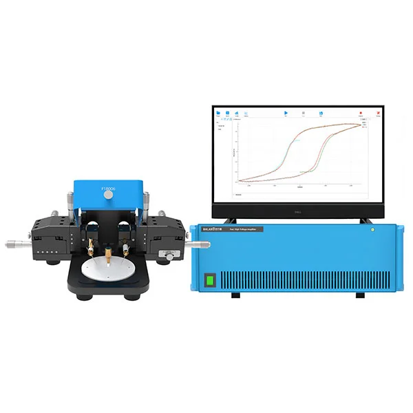
MatMeas FEAI1000 High-Precision Ferroelectric Analyzer
The MatMeas FEAI1000 is an advanced High-Precision Ferroelectric Analyzer specifically engineered for the rigorous evaluation of ferroelectric thin-film materials. Equipped with a built-in or external ±100V high-voltage amplifier, it delivers exceptional accuracy in measuring P-E hysteresis loops, spontaneous polarization, and leakage currents. Designed with proprietary high-voltage breakdown protection, it completely prevents the common catastrophic failures seen in traditional imported models. Offering measurement fidelity that directly rivals the German aixACCT TF2000 and surpassing the PolyK LY20, the FEAI1000 is the ultimate cost-effective infrastructure for dielectric functional ceramics research.
View details →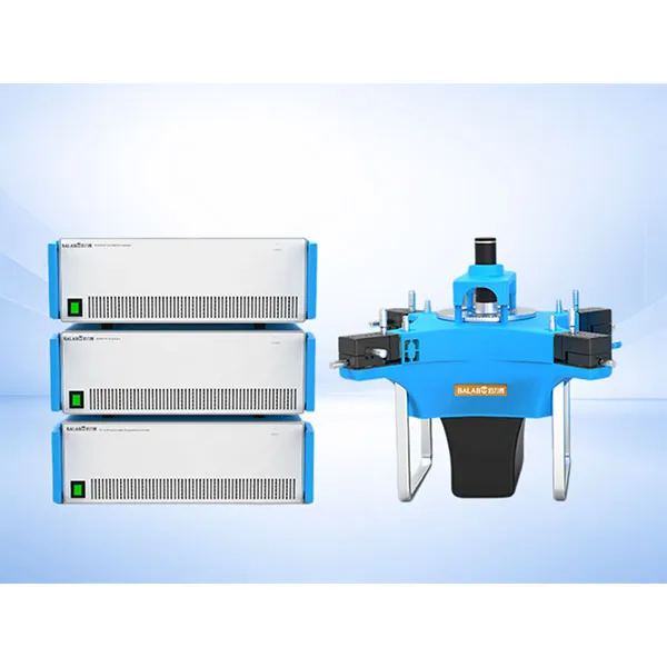
MatMeas FMS Ferroelectric Measurement Spectrometer
MatMeas High‑precision ferroelectric measurement system for hysteresis loop, fatigue testing and leakage current analysis under extreme temperatures.
View details →Request High-Precision Testing Solutions
Get expert guidance and customized instruments for your functional materials project.