Thermally Stimulated Depolarization Current Testing of Piezoelectric Ceramics
Technical News
Thermally Stimulated Depolarization Current (TSDC)—also designated in solid-state physics as Thermally Stimulated Currents (TSC) or Ionic Thermocurrents (ITC)—is an ultra-sensitive spectroscopic metrology used to investigate defect chemistry, trap depth distributions, dipole relaxation kinetics, and space-charge dynamics in functional electronic ceramics. While standard impedance spectroscopy is limited to detecting bulk relaxations with equivalent capacitances in the picofarad range, TSDC operates by sampling macroscopic depolarization currents down to the sub-picoampere (fA to pA) threshold. This provides up to three orders of magnitude higher sensitivity to dilute defect concentrations, oxygen vacancy clusters, and localized charge trapping states.
In piezoelectric and ferroelectric ceramics—including PZT, bismuth layer-structured ferroelectrics, and barium titanate—macroscopic performance is dictated by defect-domain interactions. Reversible domain wall mobility, aging rates, fatigue endurance, and high-temperature insulation degradation are directly governed by the thermodynamic depth and spatial distribution of point defect energy levels (such as ionized oxygen vacancies V_O_ddot and lead vacancy V_Pb'' complexes).
Extracting quantitative activation energies (E_a) and relaxation attempt times (tau_0) from a raw TSDC thermogram requires understanding the classical Bucci-Fieschi-Guidi (BFG) kinetic formulation, executing initial rise analysis, deconvolving multi-peak spectra, and maintaining rigorous vacuum-shielded experimental boundaries in accordance with ASTM D257 and IEEE Std 400.
Thermodynamic Theory: The Bucci-Fieschi-Guidi (BFG) Relaxation Kinetics
A standard TSDC experiment comprises four sequential experimental stages:
+---------------------------------------------------------------------------------------------------+
|                                 The Four Sequential Stages of a TSDC Run                          |
+---------------------------------------------------------------------------------------------------+
|  Stage 1: High-Temperature Polarization (T_p)                                                     |
|  Specimen heated to T_p; DC electric field E_p applied for time t_p -> dipoles align, traps fill. |
|                                                                                                   |
|  Stage 2: Cryogenic Field-Quench Freezing (T_0)                                                   |
|  Field E_p maintained while sample is rapidly quenched to T_0 (-160 C) -> defect states frozen.   |
|                                                                                                   |
|  Stage 3: Field Removal and Short-Circuit Discharge                                               |
|  Electric field removed; electrodes shorted for time t_d -> fast geometric capacitive charge drains|
|                                                                                                   |
|  Stage 4: Linear Thermal Ramp and Current Sampling (beta = dT/dt)                                 |
|  Sample heated at strict constant rate beta; picoammeter records depolarization current I(T).     |
+---------------------------------------------------------------------------------------------------+
During Stage 4, thermal energy overcomes the trapping barriers, allowing frozen dipoles to randomize and trapped space charges to release. For a single non-interacting dipolar relaxation process governed by Debye kinetics, the rate of polarization decay (dP/dt) satisfies:
dP(t) / dt = - P(t) / tau(T)
Where tau(T) is the temperature-dependent dielectric relaxation time, described by the classical Arrhenius relation:
tau(T) = tau_0 * exp(E_a / (k_B * T))
Here:
- E_a: The activation energy required for the dipole to overcome its internal reorientation barrier (or the trap depth for a localized carrier).
- tau_0: The characteristic relaxation time constant at infinite temperature (the inverse of the molecular/lattice attempt frequency, typically 1e-12 to 1e-14 seconds).
- k_B: The Boltzmann constant (8.61733e-5 eV/K).
Because temperature ramps at a constant linear heating rate (beta = dT/dt, hence dt = dT / beta), integrating the differential equation yields the polarization retention P(T) as a function of temperature:
P(T) = P_0 * exp[ - (1 / beta) * integral_{T_0}^T (1 / tau(T')) dT' ]
The observable depolarization current density J(T) flowing through the external short-circuited electrometer is:
J(T) = - dP / dt = - beta * (dP / dT) = P(T) / tau(T)
Substituting P(T) into this relation yields the celebrated Bucci-Fieschi-Guidi (BFG) equation:
J(T) = (P_0 / tau_0) * exp(- E_a / (k_B * T)) * exp[ - (1 / (beta * tau_0)) * integral_{T_0}^T exp(- E_a / (k_B * T')) dT' ]
Where P_0 is the initial frozen polarization charge density:
P_0 = (1 / beta) * integral_{T_0}^{T_end} J(T) dT
Theoretical BFG Depolarization Thermogram Profile:

Current Density J(T)
    ^                                Peak Temperature T_m
    |                                        |
    |                                       ***
    |                                      *   *  Asymmetric High-Temp
    |               Initial Rise Slope    *     * Rapid Exhaustion
    |               ln(J) vs -1/T        *       *
    |                             ****  *         *
    |                         ****     *           *
  0 +------------------------*--------*-------------*---------------------> Temperature (T)
                            T_0      T_m           T_end
The BFG curve exhibits a characteristic asymmetric bell shape:
- Low-Temperature Leading Edge: The exponential term exp(-E_a / (k_B * T)) dominates, causing current to rise steeply as thermal energy unfreezes carriers.
- Peak Maximum (T_m): Occurs where the rate of carrier release exactly balances the rapid exhaustion of the remaining frozen charge population. Setting dJ/dT = 0 yields the transcendental peak condition: T_m^2 = (beta * E_a * tau(T_m)) / k_B = (beta * E_a * tau_0 / k_B) * exp(E_a / (k_B * T_m))
- High-Temperature Trailing Edge: The integral exhaustion term dominates, causing current to plunge sharply back to zero.
Mathematical Extraction of Trap Parameters
To convert raw TSDC current peaks into quantitative physical values (E_a and tau_0), three analytical methods are utilized:
1. The Garlick-Gibson Initial Rise Method
At the beginning of the depolarization peak (temperatures well below the peak maximum, T << T_m), the total remaining polarization is virtually unchanged from its initial value: P(T) approx P_0. The second exponential integral in the BFG equation remains close to unity:
exp[ - (1 / (beta * tau_0)) * integral_{T_0}^T exp(- E_a / (k_B * T')) dT' ] approx 1
Under this boundary condition, the current density simplifies strictly to the leading Arrhenius term:
J(T) approx (P_0 / tau_0) * exp(- E_a / (k_B * T))
Taking the natural logarithm yields:
ln(J(T)) = - (E_a / k_B) * (1 / T) + ln(P_0 / tau_0)
Plotting ln(J(T)) against 1000 / T for the first 10% to 15% of the peak height produces a straight line whose slope directly yields the trap activation energy E_a:
E_a = - k_B * [ d(ln J) / d(1 / T) ]
The primary advantage of the Garlick-Gibson method is that it is completely independent of the kinetic order of the process, the heating rate beta, and any overlap on the high-temperature side of the peak.
2. The Bucci Full-Curve Area Integration Method
When a depolarization peak is isolated from adjacent transitions, the entire current thermogram can be integrated to calculate the remaining polarization P(T) at any arbitrary temperature point:
P(T) = (1 / beta) * integral_T^{T_end} J(T') dT'
Because J(T) = P(T) / tau(T), the relaxation time tau(T) at any temperature is extracted directly from the ratio of remaining peak area to instantaneous current:
tau(T) = P(T) / J(T) = [ integral_T^{T_end} J(T') dT' ] / [ beta * J(T) ]
Plotting ln(tau(T)) versus 1 / T yields a straight line across the entire peak profile, enabling simultaneous extraction of both activation energy E_a (from the slope) and the attempt time constant tau_0 (from the intercept at 1/T = 0).
3. The Kissinger Multi-Heating-Rate Method
By executing multiple TSDC runs on the same specimen at different heating rates (e.g., beta = 1, 2, 4, 8 C/min), the peak temperature shifts upward: higher heating rates provide less thermal dwell time per temperature interval, shifting T_m to higher values.
Rearranging the peak condition:
ln(beta / T_m^2) = - (E_a / k_B) * (1 / T_m) + ln(k_B / (E_a * tau_0))
A plot of ln(beta / T_m^2) versus 1 / T_m yields a straight line with slope -E_a / k_B, providing a robust cross-check that is immune to baseline electrometer offsets.
Deconvolution Matrix: Classifying TSDC Depolarization Peaks
In piezoelectric ceramics, a raw TSDC spectrum from -160 C to 450 C typically exhibits three to five overlapping current peaks. The table below compiles diagnostic rules used to classify each physical mechanism.
| TSDC Peak Classification | Typical Temperature Regime (PZT) | Physical Microscopic Mechanism | Diagnostic Test Behavior | Activation Energy (E_a) Range |
|---|---|---|---|---|
| Low-Temp Dipolar Peak (P1) | -100 C to 0 C (Cryogenic) | Localized reorientation of defect dipoles (e.g., V_Pb'' - V_O_ddot) | Peak area scales strictly linearly with polarization field E_p | 0.20 eV to 0.45 eV (shallow trap) |
| Domain De-Aging Peak (P2) | +50 C to +150 C (Sub-Curie) | 90-degree and 180-degree ferroelectric domain boundary relaxation | Peak area exhibits saturation threshold; sensitive to mechanical stress | 0.60 eV to 0.95 eV (domain pinning) |
| Space-Charge / Oxygen Vacancy Peak (P3) | +180 C to +280 C (Pre-Curie) | Detrapping and drift of mobile oxygen vacancies to grain boundaries | Peak temperature T_m shifts with polarization temperature T_p | 0.90 eV to 1.30 eV (ionic hopping) |
| Curie Phase Transition Peak (P4) | +320 C to +360 C (At T_c) | Annihilation of spontaneous ferroelectric polarization at Curie point | Enormous current spike; coincides exactly with dielectric peak | Apparent E_a > 3.0 eV (thermodynamic) |
| Electrode Interfacial Charge Peak (P5) | > +380 C (Post-Curie) | Discharge of accumulated space charge at blocking electrode contacts | Peak shape depends strongly on electrode material (Au vs Pt) | 1.40 eV to 2.00 eV (Schottky barrier) |
Experimental Challenges: Sub-Picoampere Current Acquisition
Measuring TSDC currents in piezoelectric ceramics involves detecting currents between 10 femtoamperes (1e-14 A) and 100 nanoamperes (1e-7 A) while ramping temperature across a 600 K span. Standard laboratory furnaces fail completely due to three destructive noise sources:
- Triboelectric Micro-Fretting Noise: As furnace fixtures heat and expand, probe needles slide microscopically across metal electrode pads. This mechanical sliding friction generates triboelectric charge spikes (pC range) that completely obliterate sub-picoampere depolarization signals.
- Atmospheric Moisture Condensation: When cooling below 0 C under ambient air, humidity freezes into ice. Upon reheating, melting ice generates massive electrochemical false current peaks near 0 C that obscure dipolar relaxation.
- Furnace AC Electromagnetic Induction: 50/60 Hz AC currents powering resistive heating elements induce displacement currents into unshielded sample leads, swamping DC electrometers.
The table below outlines instrumentation requirements necessary to eliminate these measurement artifacts.
| Experimental Parameter | Standard Thermal Fixture (Inadequate) | High-Performance TSDC System (Audit-Compliant) |
|---|---|---|
| Vacuum Atmosphere | Ambient atmospheric air or loose nitrogen purge | High vacuum (< 1e-4 mbar) pumped via turbomolecular station |
| Low-Temperature Limit | 0 C to -20 C (limited by chiller) | -160 C (continuous liquid nitrogen cryostat injection) |
| Vibration Isolation | Rigid bolted stage (transmits building vibrations) | Built-in pneumatic air-shock anti-vibration damping stage |
| Electrometer Noise Floor | 100 fA to 1 pA RMS (standard DMM / picoammeter) | < 1 fA RMS (triaxial guarded electrometer front-end) |
| Probe Mechanical Contact | Spring-loaded pogo pins (slide during expansion) | Micro-manipulated tungsten probes on compliant flexures |
| Thermal Lag Control | Chamber air thermocouple (severe thermal lag) | Coplanar calibrated platinum RTD directly adjacent to sample |
| Electrode Guarding | Two-wire unguarded coaxial line | Full triaxial guarding matching ASTM D257 geometry |
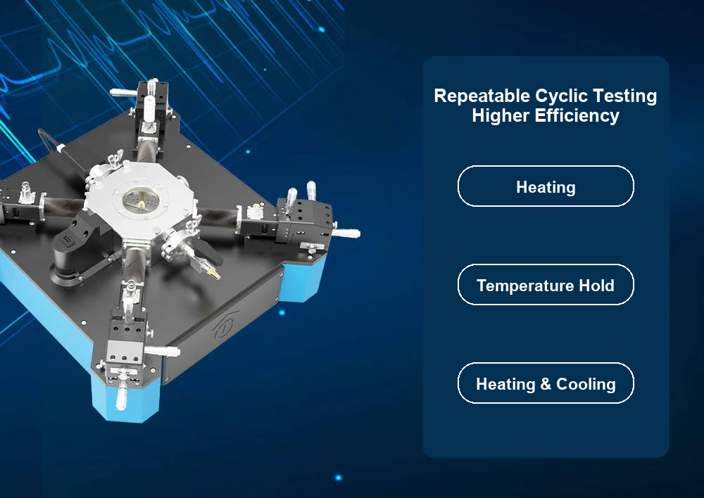
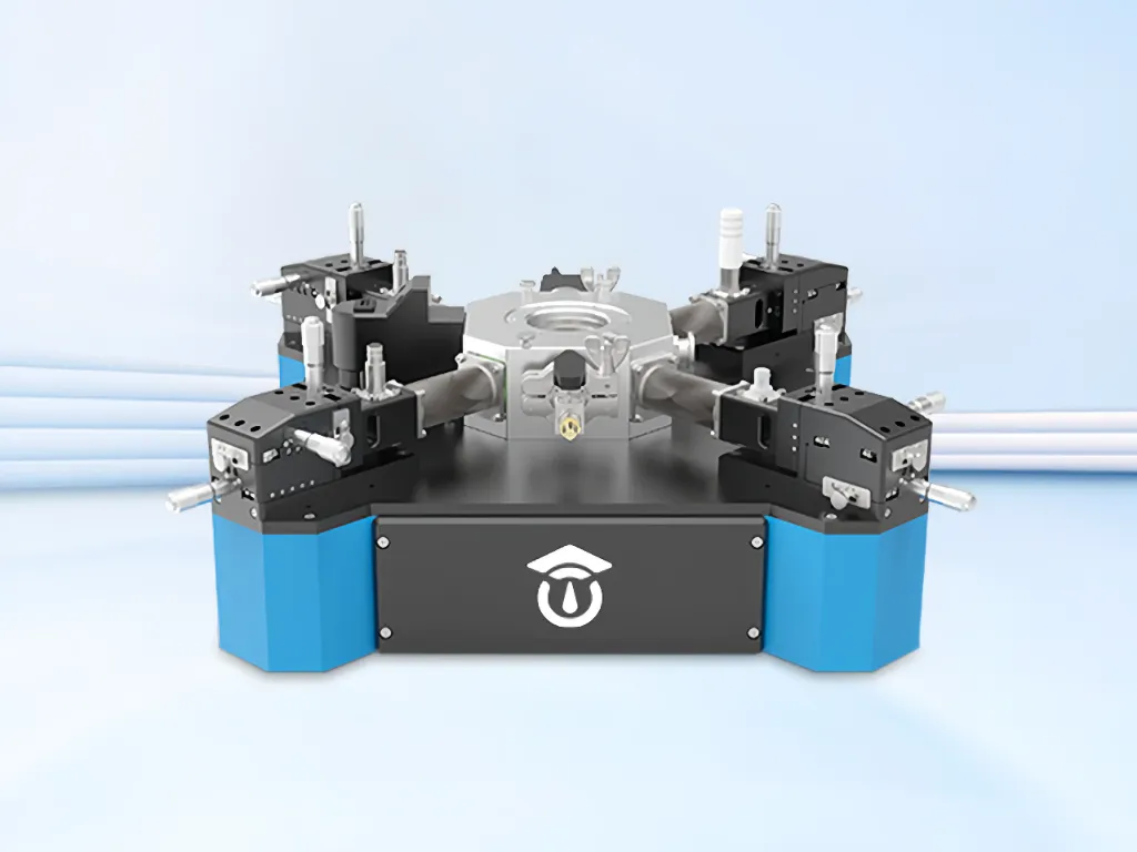
To satisfy these rigorous criteria, materials researchers deploy the MatMeas CPS-7000 Cryogenic Vacuum Probe Station. The CPS-7000 integrates liquid-nitrogen cooling down to -160 C and controlled resistive heating up to 450 C under high vacuum. Uniquely equipped with a proprietary built-in pneumatic air shock anti-vibration platform, it completely eliminates mechanical probe chatter and triboelectric jumping noise, enabling clean, artifact-free acquisition of sub-picoampere defect spectra.
Best-Practice Laboratory SOP for Piezoelectric Ceramic TSDC
To produce peer-reviewed, reproducible TSDC thermograms, adhere to the following experimental procedure:
- Sample Preparation and Sizing:
- Fabricate circular ceramic discs (diameter 10 mm to 15 mm, thickness 0.5 mm to 1.0 mm) with mirror-polished parallel faces (Ra < 0.2 um).
- Deposit thin-film gold or platinum electrodes (thickness 100 nm to 150 nm) using magnetron sputtering. Ensure a clean 1.5 mm uncoated annular margin around the perimeter to suppress edge flashover during Stage 1 poling.
- Loading into High-Vacuum Cryostat:
- Mount specimen onto the vacuum thermal chuck of the probe station.
- Land micro-probes on the center of the top electrode with minimal contact force to avoid indenting the film.
- Evacuate the vacuum chamber to a base pressure < 1e-3 mbar before initiating thermal cycling to ensure complete desorption of surface moisture.
- Stage 1: Polarization (T_p, E_p, t_p):
- Heat specimen to the chosen polarization temperature T_p (e.g., 150 C for PZT, chosen below T_c).
- Apply a calibrated DC electric field E_p (typically 0.5 kV/mm to 2.0 kV/mm, verified below dielectric breakdown).
- Dwell under active field for t_p = 30 minutes to allow mobile defect dipoles to attain thermodynamic equilibrium orientation.
- Stage 2: Cryogenic Quenching (T_0):
- While maintaining the full DC electric field E_p, initiate rapid liquid nitrogen cooling.
- Quench the sample at >= 10 C/min down to cryogenic temperature T_0 = -160 C (113 K) to immobilize the aligned defect states.
- Stage 3: Depolarization and Short-Circuiting (t_d):
- Turn off the DC voltage supply and short the electrometer input across the specimen through a 1-megaohm current-limiting resistor.
- Maintain the short circuit at T_0 for t_d = 10 minutes to drain all fast geometric capacitive charge (Q = C * V).
- Stage 4: Controlled Linear Reheating and Acquisition (beta):
- Connect the specimen to the triaxial electrometer front-end.
- Ramp temperature upward at a constant linear rate beta = 3.0 C/min (+/-0.05 C/min) up to 400 C.
- Sample depolarization current continuously at 1 Hz, logging real-time current, sample temperature, and time.
- Baseline Subtraction and Peak Deconvolution:
- Cool the specimen back down and immediately execute a second identical heating run without applying an electric field (zero-bias rerun) to record the parasitic thermoelectric and fixture baseline current.
- Subtract this baseline from the Stage 4 spectrum.
- Perform Garlick-Gibson initial rise analysis and BFG non-linear least squares fitting to extract E_a and tau_0 for each deconvolved peak.
Frequently Asked Questions (FAQ)
What is the fundamental difference between TSDC and standard AC dielectric loss (tan delta) spectroscopy?
Dielectric loss spectroscopy measures the phase lag of dipole oscillations under a continuous alternating AC electric field at fixed isothermal temperatures. At low frequencies or high temperatures, large ohmic conduction currents (sigma_dc / (epsilon_0 * omega)) completely overwhelm weak dielectric absorption peaks. In contrast, TSDC applies a DC polarizing field, quenches the defect state, discharges all conductive charges, and measures current during non-isothermal heating in the absence of an external field. Because no external voltage is applied during measurement, steady-state DC leakage is fundamentally absent, allowing TSDC to resolve ultra-weak defect relaxations with 100 to 1,000 times higher sensitivity than AC impedance analyzers.
How can an operator distinguish between an intrinsic dipolar relaxation peak and a space-charge trapping peak?
To differentiate dipolar from space-charge peaks, two diagnostic tests are standard:
- Linearity with Polarization Field (E_p): The area under a dipolar relaxation peak (P_0) is governed by Langevin-Debye statistics and scales strictly linearly with applied electric field (P_0 proportional to E_p) up to high fields. Space-charge peaks, however, show non-linear saturation as trap levels become fully occupied, or sudden exponential growth if injection occurs.
- Thermal Windowing (Fractional Polarization): Apply the field E_p only during a narrow temperature window (Delta T = 5 C) during cooling, followed by short-circuiting. Dipolar peaks will shift and isolate into single elementary Debye peaks, whereas distributed space-charge traps decompose into broad continuous energy bands.
Why does a TSDC peak temperature (T_m) shift to higher temperatures when the heating rate is increased?
The peak temperature T_m represents the point where the rate of thermal release equals the exhaustion rate of remaining frozen dipoles. When the linear heating rate (beta = dT/dt) is increased, the sample spends less physical time within each temperature interval. Consequently, frozen dipoles do not have sufficient time to relax at their lower equilibrium temperatures. The relaxation kinetics are pushed to higher temperatures before the peak exhaustion condition is reached, causing T_m to shift upward according to the Kissinger relation: ln(beta / T_m^2) proportional to - 1 / T_m.
Request High-Precision Testing Solutions
Get expert guidance and customized instruments for your functional materials project.